This article explains how to use Semrush keyword data to create a time series chart in Google Sheets that more accurately reflects monthly search demand trends. Keep in mind search volume itself isn’t a reliable metric: treat it as an estimate and use it to make comparisons and see patterns.
Data Scaling for the Rest of Us
Tyler Einberger used this process when an ecommerce client asked how search demand for several products had been trending over past months. He answered the question with a big clear chart, and documented the visualization process for the rest of us at Momentic to use. I took his documentation and turned it into these illustrated step-by-step instructions.
Tools like Semrush, Google Trends and Keyword Planner provide relative trend values for keywords: they show how a keyword's popularity changes over time. But that’s not helpful when you export the data to a spreadsheet, because those monthly trend values don't represent a number of searches per month.
To make the exported search trend data more useful, we’re going to use ‘Multiplier K’ to adjust the relative trend values for each keyword so they align with monthly search volume. Multiplier K is the magic sauce that transforms relative changes into absolute values, giving you a more accurate picture of month-by-month search demand.
If that sounds daunting, don’t worry. Data scaling is not in my wheelhouse and I had doubts my first time through. I promise if you follow along one step at a time it will work!
To use this guide, you’ll need:
- Access to Keyword Overview > Bulk Analysis in Semrush
- Basic working knowledge of Google Sheets
- Understanding of time series data and charts
Step One: Export Data from Semrush
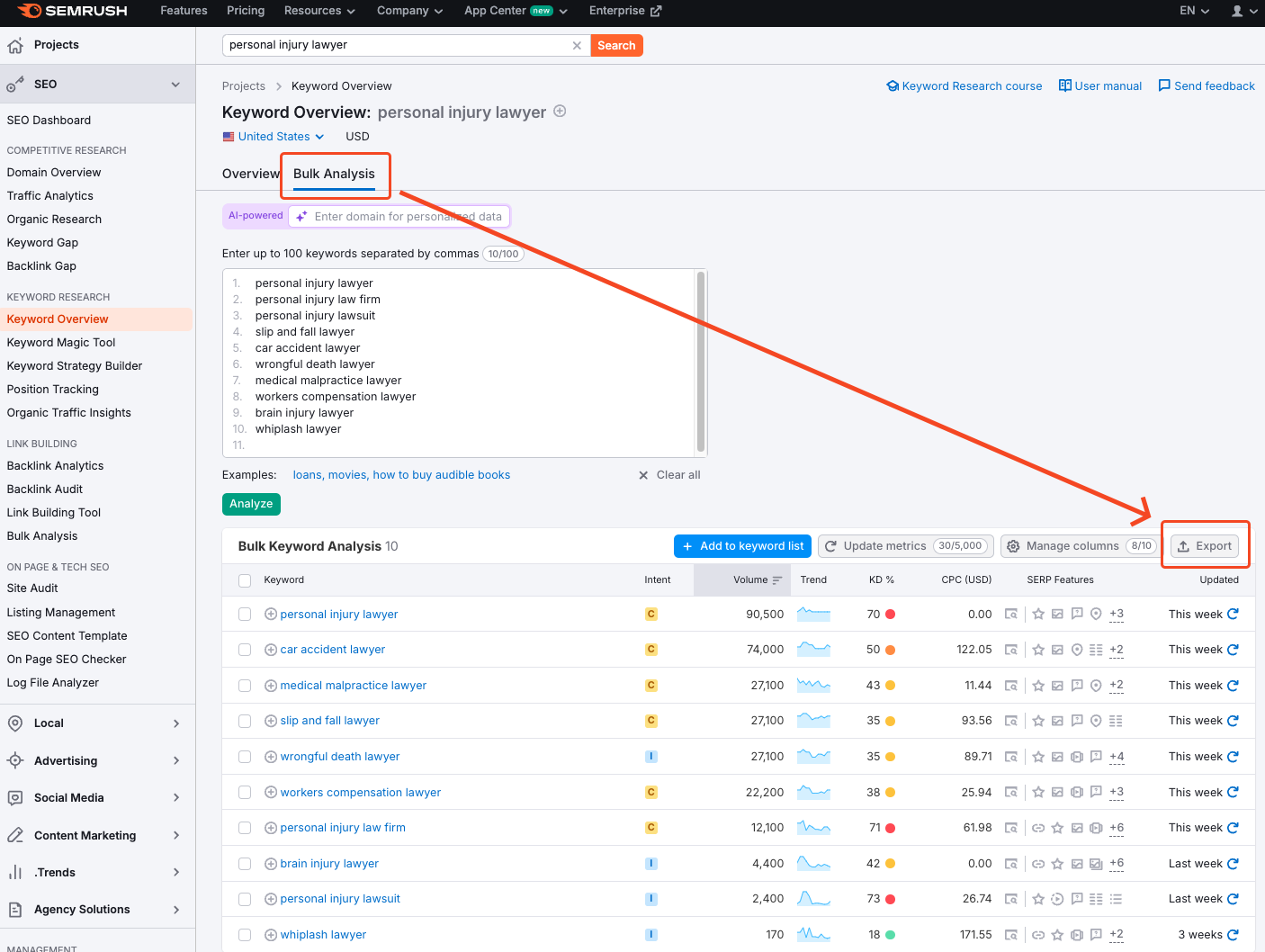
<div class="post-action">Go to the Keyword Overview tool in Semrush.</div>

You won’t see the Bulk Analysis option until after you enter one or more keywords. Because each keyword will be represented as a line in a time series chart, you should probably limit your list to around ten.
It’s also helpful if the keywords don’t have wildly different search volumes, since they’ll be visualized on a shared scale. For example, if some your keywords have search volumes around 150K/month and others have search volumes around 50/month, some of the lines will be hard to see in the chart.
<div class="post-action">After analysis, click Export. Choose CSV as the format. Save file to your computer.</div>
Step Two: Import Data into Google Sheets
Create a new Google Sheet and import the CSV file.
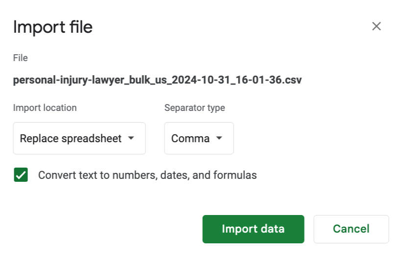
<div class="post-action">Click on File > Import. Click on the Upload tab and browse to find the CSV, or drag and drop.</div>
Import location = Replace spreadsheet
Separator type = Comma
<div class="post-action">Leave the box checked that says “Convert text to numbers, dates, and formulas”. Then click Import data.</div>
Step Three: Process the Trend Data
Next, we’re going to split the trend data into multiple columns.
<div class="post-action">Select the Trend column. Click on Data > Split text to columns.</div>
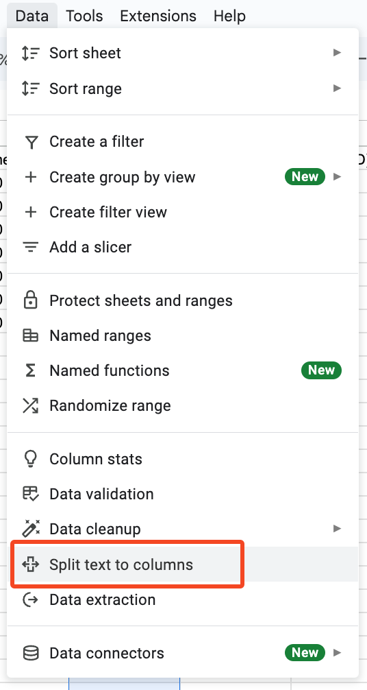
<div class="post-action">A small gray Separator menu will appear at the bottom of the column. Choose Custom. Enter a comma (,) in the field that appears.</div>
Presto: now trend data is split up across twelve columns. You need to give each column a name in the header row. Each column should be named after a month/year, in sequence from earliest to latest.
Semrush keyword trends are analyzed over the previous 12 months, not including partial months. Start with the far right column and enter the date of the most recent full month. Then work backwards, right to left.
In this example, keyword trend data was exported from Semrush towards the end of October 2024. So the most recent complete month was September 2024, and trend data goes back through October 2023.
<div class="post-action">Pro tip: You’ll need to replace the original “Trend” column header with a month/year also.</div>

Review your columns. From left to right, they should now read:
- Keyword
- Intent
- Volume (rename to “Average Monthly Demand”)
- Month/Year (12 of these)
- Keyword Difficulty
- CPC
- SERP Features
- Multiplier K (you need to add this column - it’ll be calculated next!)
Step Four: Calculate Multiplier K
Multiplier K is a formula that adjusts the monthly trend values to align with a reference point—in this case, average monthly demand (aka search volume).
Before we can use Multiplier K, we need to find the average of each keyword’s monthly trend values.
<div class="post-action">Find an empty cell in your first keyword row, somewhere off to the right. Enter this formula: =AVERAGE(D2:O2)</div>
D2 and O2 are the cells used in this example - if your sheet populated differently, you'll need to replace the cell designators in parentheses with those of the first and last cells containing monthly trend values for that keyword.
<div class="post-action">Once the formula’s been applied in the first keyword row, drag it down to apply it to all of them.</div>

<div class="post-action">Highlight all those cells you just filled in with the formula. Hit Command + C then Command + V (Mac) or Control + C then Control + V (PC). </div>
You’re copying and pasting right back in the same place.
<div class="post-action">After pasting, select Paste values only from the little clipboard menu in the lower right corner of the highlighted cells.</div>
Now the cells are filled in with values, instead of a formula, which is important for the next step.

<div class="post-action">Go to the first cell in your Multiplier K column. Enter this formula: =C2/T2</div>
Replace cell designators in formula if needed:
- C2 is the average monthly demand for the keyword as exported from Semrush.
- T2 is the average of the monthly trend values for that keyword (it’s what we just calculated).
<div class="post-action">Apply that C2/T2 formula to all the cells in the Multiplier K column.</div>
Congratulations: you've calculated Multiplier K for each keyword!
<div class="post-action">Do the same copy/paste maneuver as before, and paste values only.</eiv>
Step Five: Adjust Monthly Trend Values
Next we’re going to use Multiplier K to scale each monthly trend value.
<div class="post-action">First, make a copy of the monthly trend values for each keyword (with header row) and paste it in a fresh area lower down in the sheet, aligned with the same columns.</div>
<div class="post-action">In the recently pasted data, in the first cell of the first month, enter this formula: =D2*$S2</div>
Replace cell designators in the formula if needed: In this example:
- D2 is the first keyword’s trend value for the first month.
- S2 is the cell that has that keyword’s Multiplier K value.
<div class="post-action">Apply that formula across all the monthly columns for that keyword.</div>
In this example, they go from D15 to O15, indicated by the orange arrow:
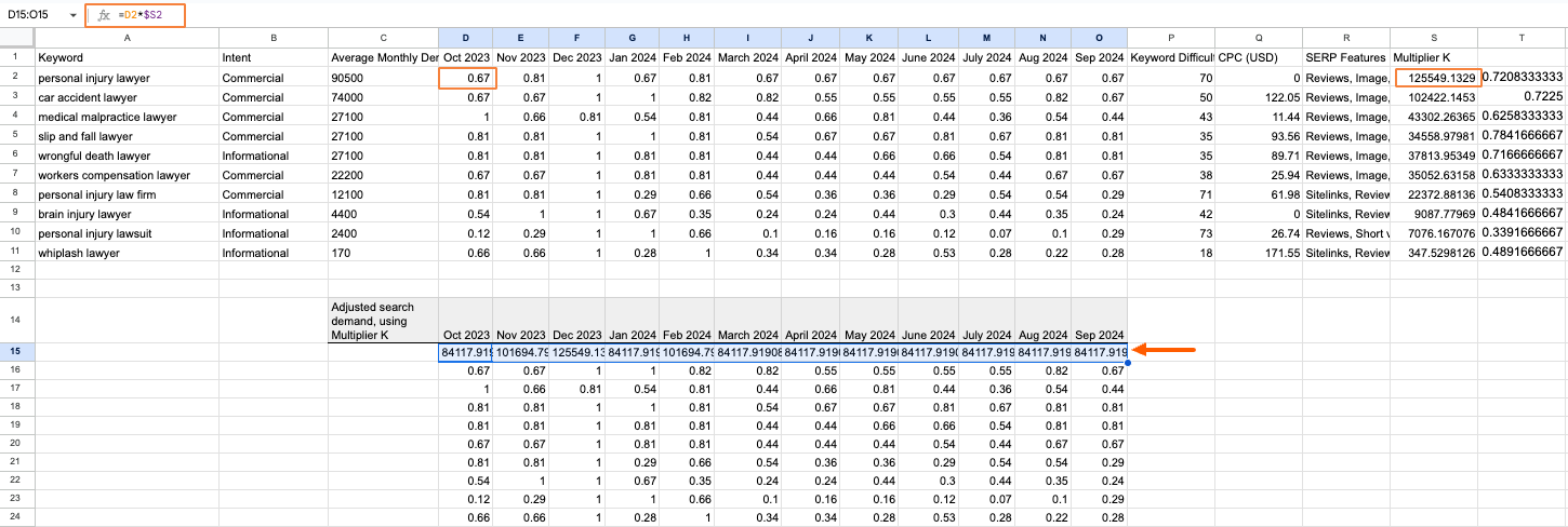
<div class="post-note-cute">Those adjusted monthly trend values now represent estimated search demand for each month, scaled appropriately. This is the data we’ve been working toward!</div>
<div class="post-action">Now do the same thing for the monthly trend values for the rest of the keywords.</div>
One more time: copy/paste all of them back in the same place, and paste values only because we need to use values (not formulas) to make a chart out of this.
Step Six: Create a Time Series Chart
<div class="post-action">Put the keywords next to their adjusted monthly trend values.</div
You can either replace the original trend values with the adjusted ones you just made, or copy the keywords and put them alongside the adjusted values.
<div class="post-action">Select all the keywords, adjusted monthly trend values & header row. Click Insert > Chart.</div>
A Chart Editor panel appears on the right, and a chart appears in the sheet:
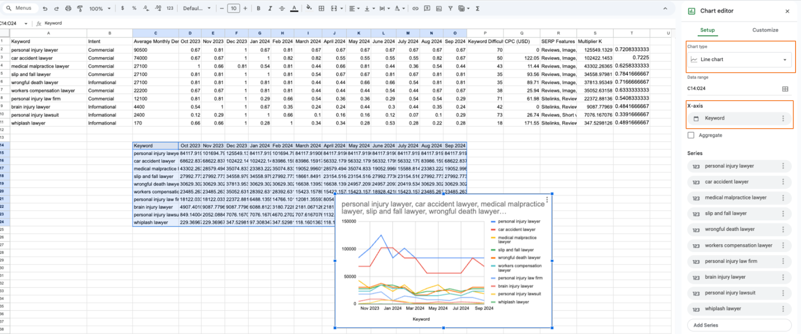
<div class="post-action">Use the Customize tab in the Chart Editor to choose a chart type, smooth the lines, pick different colors, adjust the X-axis and Y-axis, add a title, data labels, legend etc until you’re happy with it.</div>
And that’s it! Now you have a nice visual showing how monthly search demand has fluctuated for your set of keywords over the past 12 months.
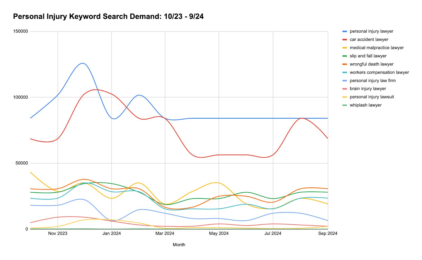
Note: I used personal injury keywords for the example since we don’t have any lawyer/law firm clients - but the data is real!
Use Cases
- Give clients or internal stakeholders a high-level view of how search demand for products & services has been trending
- Plan content strategy (both publication & refreshing) to align with periods of higher search volume
- Identify keywords with consistent search volume that have potential for long-term SEO efforts
- Discover keywords with declining search volume (so you can include other variations in your keyword strategy)
- Adjust paid campaigns based on anticipated search demand fluctuations
- Independent analysis and visualization of search demand trends
- Manipulate and present data outside of the Semrush platform
<div class="post-note-cute">If you need help finding historical keyword search volumes, creating visualizations for decision makers, or have questions about anything Search or keyword related, that’s 100% our jam, so don’t hesitate to reach out: <a href="mailto:info@momenticmarketing.com">info@momenticmarketing.com</a></div>
Bonus: Multipliers in Data Scaling
Multiplier K is a scaling factor used to convert relative values (like whether search demand is “higher” or “lower” from one month to the next) into absolute figures (like an actual number of searches each month).
Relative values are also referred to as index numbers or normalized scores. They only represent a data point’s relative position within the dataset. To do meaningful comparisons and analysis, a multiplier is used.
Mathematically, the multiplier is calculated as:
K=Actual Total or Average ValueSum or Average of Relative ValuesK = \frac{\text{Actual Total or Average Value}}{\text{Sum or Average of Relative Values}}K=Sum or Average of Relative ValuesActual Total or Average Value
This formula makes sure the scaled (adjusted) data maintains the original distribution or pattern of the relative values, while aligning with a known total or average. In other words, it acts as a grounding rod for the monthly ups and downs so you can see a real number increasing and decreasing (instead of just how much higher or lower it is compared to the previous month).
Applications of Multipliers
- Economics: Adjusting index numbers like the Consumer Price Index (CPI) to reflect actual price levels
- Finance: Scaling normalized financial indicators to match actual revenue or profit figures
- Market Research: Converting survey percentages into projected population counts
- Data Analytics: Transforming machine learning output probabilities into real-world quantities
In all these scenarios, the multiplier serves as a bridge between relative indicators and absolute measures, allowing for more accurate analysis and interpretation.


.png)


